Sampling schemes

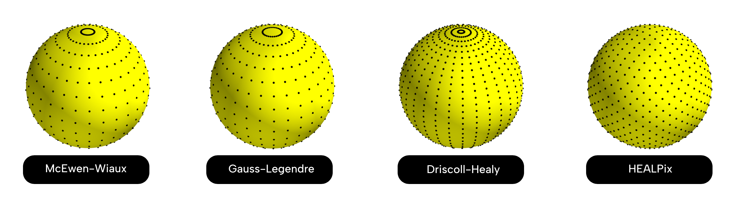
The structure of the algorithms implemented in S2FFT can support a number of sampling schemes, which we give a brief overview of here. An at-a-glance summary of the differences between the supported sampling schemes is also provided in the table below, with further information available in the dedicated section for each scheme. A more thorough overview of the schemes can be found in section 4.2 of Price & McEwen (2025).

We adopt the usual S2FFT conventions for spherical coordinates; \(\theta\in[0, \pi]\) (colatitude) and \(\varphi\in[0,2\pi)\) (longitude), with \(\theta_t\) and \(\varphi_p\) being the discretised samples (indexed by $t$ and $p$) drawn by the sampling scheme. We denote by $L$ the band-limit of the signals we are considering.

At-a-glance comparison of sampling schemes

Scheme	API string	Number of sample points [1]	Equi- angular	Equal region area	Sampling theorem
McEwen & Wiaux (MW)	"mw"	\(L\times(2L-1)\)	Yes	No	Yes
McEwen & Wiaux with Symmetric Sampling (MWSS)	"mwss"	\((L+1)\times 2L\)	Yes	No	Yes
Driscoll & Healy (DH)	"dh"	\(2L\times (2L-1)\)	Yes	No	Yes
Gauss-Legendre (GL)	"gl"	\(L\times (2L-1)\)	No	No	Yes
HEALPix	"healpix"	$12 N_{side}^2$	No	Yes	No

Specifying sampling schemes in S2FFT

All transforms implemented by S2FFT must be informed of which sampling scheme has been used to draw signal values on the sphere (with the default typically being the MW scheme). This is specified by providing the sampling argument to the transform in question, when the transform is called. Other utility functions also accept a sampling argument, which is used to adjust the behaviour of the function accordingly based on the sampling scheme being used.

As a (somewhat trivial) example to illustrate these conventions, we will generate the \(\theta_t, \varphi_p\) sample grids for the MW and GL schemes. Then, we will sample a known signal at these grid points, and have S2FFT perform forward transforms on the resulting samples in accordance with the sampling schemes. We will then confirm that the harmonic coefficients computed from each set of sample data are close, to within computational error. First, we must perform some setup:

import jax
jax.config.update("jax_enable_x64", True)

import jax.numpy as jnp

from s2fft.transforms.spherical import forward, inverse
from s2fft.sampling.s2_samples import thetas, phis_equiang

L = 512

def signal(theta, phi):
    """Our known signal function, that we will 'sample' from."""
    return jnp.sin(theta)**2 * jnp.sin(phi)

We can generate arrays containing the \(\theta_t\) and \(\varphi_p\) sample coordinates for the MW and GL schemes using thetas() and phis_equiang(). Passing the sampling argument to each of these functions specifies which scheme we want to generate sample coordinates for. We then evaluate our known signal function at the sample points to generate our ‘samples’ / ‘observations’ for each scheme.

# Generate (theta, phi) points used by the MW scheme
mw_thetas, mw_phis = thetas(L, sampling="mw"), phis_equiang(L, sampling="mw")
# Generate (theta, phi) points used by the GL scheme
gl_thetas, gl_phis = thetas(L, sampling="gl"), phis_equiang(L, sampling="gl")

# We now pretend we have two different observations of this signal,
# but which sampled it using different schemes.
mw_signal_samples = signal(*jnp.meshgrid(mw_thetas, mw_phis, indexing='ij'))
gl_signal_samples = signal(*jnp.meshgrid(gl_thetas, gl_phis, indexing='ij'))

Now that we have two sets of samples from the same signal, we can forward transform obtain the harmonic coefficients. In each case, we need to specify which sampling scheme was used to obtain the data, by passing the sampling argument to the forward() transform when we call it. Our signal is not band-limited, but using by using a suitably high band-limit we expect the computed harmonic coefficients for both transforms to be close.

# Forward-transform the same signal, but sampled using different schemes
flm_mw = forward(mw_signal_samples, L, sampling="mw", method="jax")
flm_gl = forward(gl_signal_samples, L, sampling="gl", method="jax")

# The norm of the greatest different between harmonic coefficients
# is approximately 2e-8 with L = 512.
jnp.assert_allclose(flm_mw, flm_gl)
print(f"max| flm_mw - flm_gl | = {jnp.max(jnp.abs(flm_mw - flm_gl)):.5e}")
# Output: max| flm_mw - flm_gl | = 2.03065e-08

Sampling schemes

McEwen & Wiaux (MW)

The MW sampling theorem reduces the Nyquist rate on the sphere by a factor of two compared to the DH scheme, halving the number of spherical samples required.

It also requires fewer sampling points than the GL scheme, though asymptotically the number of sampling points used by GL is the same as MW.

Sample positions are defined by

\[\begin{split}\theta_t &= \frac{\pi (2t+1)}{2L-1}, &\quad t\in\lbrace 0,1,...,L-1 \rbrace, \\ \varphi_p &= \frac{2\pi p}{2L-1}, &\quad p\in\lbrace 0,1,...,2L-2\rbrace.\end{split}\]

The scheme uses an array of size \(L \times (2L-1)\) to store the signal. However, total number of distinct sites on the sphere used by this sampling scheme is \(N_{MW} = (L-1)(2L-1)+1 \sim 2L^2\).

Further information; McEwen & Wiaux (2012).

McEwen & Wiaux with Symmetric Sampling (MWSS)

This sampling scheme uses slightly more samples than MW, requiring an array holding \((L+1)\times 2L\) elements (with $2(L^2 - L + 1)$ independent degrees of freedom). Asymptotically, we still only require \(\sim 2L^2\) elements in memory as $L$ increases. In exchange for slightly higher memory usage, the sample locations possess antipodal symmetry.

Sample positions are defined by

\[\begin{split}\theta_t &= \frac{2\pi t}{2L}, &\quad t\in\lbrace 0,1,...,L \rbrace, \\ \varphi_p &= \frac{2\pi p}{2L}, &\quad p\in\lbrace 0,1,...,2L-1\rbrace.\end{split}\]

Further information; Ocampo, Price, & McEwen (2023).

Driscoll & Healy (DH)

Sample positions are defined by

\[\begin{split}\theta_t &= \frac{\pi (2t+1)}{4L}, &\quad t\in\lbrace 0, 1, ..., 2L-1\rbrace, \\ \varphi_p &= \frac{2\pi p}{2L-1}, &\quad p\in\lbrace 0, 1, ..., 2L-2\rbrace.\end{split}\]

This requires \(2L \times (2L-1) \sim 4L^2\) elements to be held in memory, and since the poles are not sample points, the same number of independent degrees of freedom to represent the signal.

Further information; Driscoll & Healy (1995), (however it should be noted that S2FFT adopts the \(\theta\) positions given in Healy et al. (2003) and a slightly more efficient \(\varphi\) sampling scheme).

Gauss-Legendre (GL)

The GL sampling theorem also requires an array of \(L\times (2L-1) \sim 2L^2\) elements to represent the signal. Like DH, there is no redundancy in samples at the poles, so the same number of independent degrees of freedom are needed.

The \(\theta_t\) are determined by the roots of the Legendre polynomials of order $L$, whilst the \(\varphi_p\) are defined by

\[\varphi_p = \frac{2\pi p}{2L-1}, \quad p\in\lbrace 0, 1, ...,2L-2\rbrace.\]

Further information; Gauss-Legendre (1986).

HEALPix

HEALPix sampling provides regions (pixels) of equal areas which can have many practical advantages. Unlike the other schemes, the sample points do not get denser as one approaches the poles, for example.

However, HEALPix sampling does not exhibit a sampling theorem and so round-tripping through the corresponding harmonic transforms does not recover the original signal or coefficients to machine precision but instead exhibits some non-negligible error. An iterative refinement scheme can be applied to the forward transform to reduce this round-trip error at the cost of additional computation. This can be applied in S2FFT’s forward transforms by setting the iter argument to the number of iterations to perform, with more iterations giving a smaller round-trip error.

A HEALPix grid is defined by a resolution parameter $N_{side}$, requiring $12 N_{side}^2$ elements (and independent degrees of freedom) stored in memory. Given a resolution parameter, the grid will contain $N_{hp} = 12 N_{side}^2$ regions of the same area \(\frac{\pi}{3N_{side}^2}\). The regions will be laid out on $4N_{side}-1$ iso-latitude rings, and the distribution of regions will be symmetric about the equator. For the equations defining the exact positioning of the regions, their centres, their boundaries, and how they are organised into an array, see section 5 of Gorski et al. (2005).

Further information; Gorski et al. (2005).

Footnotes

[1]

The “number of sample points” listed here refers to the size of the array recording sample values in memory. This is distinct from the “number of independent degrees of freedom” (the “number of sites on the sphere that we are required to sample”) to represent a signal, since many sampling schemes have overlapping sample points at the north (\(\theta=0\)) and south (\(\theta=\pi\)) poles. Both values are quoted in the corresponding section for each scheme, but the table only lists the former (size of the array representing a signal).