Spherical harmonic transform

This tutorial demonstrates how to use S2FFT to compute spherical harmonic transforms.

If you are working on this notebook in Google Colab; you will need to have Google Colab install cartopy, s2fft and pyssht, as well as fetch the data we’ll be using. You can do this by adding a cell to the top of the notebook with the following content:

!pip install cartopy s2fft pyssht &> /dev/null
!mkdir data/
!wget https://github.com/astro-informatics/s2fft/raw/main/examples/data/Gaia_EDR3_flux.npy -P data/ &> /dev/null

and then running that cell.

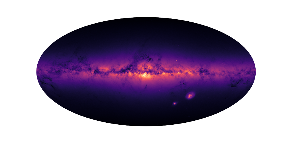
In this example we will adopt the sampling scheme of McEwen & Wiaux (2012). First let’s load an input signal that is sampled on the sphere with this sampling scheme.

import jax

jax.config.update("jax_enable_x64", True)

import cartopy.crs as ccrs
import numpy as np
from matplotlib import pyplot as plt

import s2fft

sampling = "mw"
f = np.load("data/Gaia_EDR3_flux.npy")
L = f.shape[0]

Let’s look at the input signal:

plt.figure(figsize=(10, 5))
ax = plt.axes(projection=ccrs.Mollweide())
im = ax.imshow(f, transform=ccrs.PlateCarree(), cmap="magma")
plt.axis("off")
plt.show()

Computing the forward spherical harmonic transform

Let’s now run the JAX function to compute the spherical harmonic transform of this map.

flm = s2fft.forward_jax(f, L)

If you are planning on applying this transform many times (e.g. during training of a model) we recommend precomputing and storing some small arrays that are used every time. This trades off additional memory usage for enhanced speed and should be fine at small and moderate bandlimits L.

To do this simply compute these and pass as a static argument.

precomps = s2fft.generate_precomputes_jax(L, forward=True)
flm_pre = s2fft.forward_jax(f, L, precomps=precomps)

Computing the inverse spherical harmonic transform

Let’s run the JAX function to compute the inverse spherical harmonic transform to get back to the input map.

f_recov = s2fft.inverse_jax(flm, L)

Again, if you are planning on applying this transform many times we recommend precomputing and storing some small arrays that are used every time. Recall, this trades off additional memory usage for enhanced speed and should be fine at small and moderate bandlimits L.

To do this simply compute these and pass as a static argument.

precomps = s2fft.generate_precomputes_jax(L, forward=False)
f_recov_pre = s2fft.inverse_jax(flm_pre, L, precomps=precomps)

Computing the error

Let’s check the associated error, which should be close to machine precision for the sampling scheme used.

print(f"Mean absolute error = {np.nanmean(np.abs(f_recov - f))}")
print(f"Mean absolute error using precomputes = {np.nanmean(np.abs(f_recov_pre - f))}")

Mean absolute error = 4.2080013578407947e-13
Mean absolute error using precomputes = 4.2080013578407947e-13