Understanding spherical harmonics

Spherical harmonics are the spherical counterpart of Fourier modes. Just as Fourier modes provide a basis for representing periodic functions, spherical harmonics provide a basis for representing functions defined on the sphere.

This tutorial introduces their main mathematical properties, visualises some basis functions, and shows how S2FFT decomposes a signal into spherical harmonic coefficients.

If you are working on this notebook in Google Colab, you will need to have Google Colab install s2fft. You can do this by adding a cell to the top of the notebook with the following content:

!pip install cartopy s2fft &> /dev/null

and then running that cell.

Spherical coordinates

A point on the unit sphere is described by two angles:

• \(\theta \in [0,\pi]\) is the colatitude, measured down from the north pole.

• \(\phi \in [0,2\pi)\) is the longitude around the sphere, measured eastward from a reference meridian.

We write a signal on the sphere as \(f(\theta,\phi)\). Depending on the application, it could represent quantities such as temperature, elevation, or radiation intensity.

Spherical harmonics

The spherical harmonic \(Y_{\ell m}(\theta,\phi)\) is indexed by two integers:

• The degree \(\ell=0,1,2,\dots\) controls its overall angular scale.

• The order \(m=-\ell,\dots,\ell\) controls its variation with longitude.

A spherical harmonic can be written as

\[Y_{\ell m}(\theta,\phi) = N_{\ell m} P_{\ell}^m(\cos\theta) \exp(i m\phi),\]

where \(N_{\ell m}\) is a normalisation constant, \(P_{\ell}^{m}\) is an associated Legendre polynomial controlling variation with colatitude, and \(\exp(i m\phi)\) controls variation with longitude. Consequently, spherical harmonics are generally complex-valued.

Orthonormality

The surface-area element on the unit sphere, also called the solid-angle element, is

\[\mathrm{d}\Omega = \sin\theta \ \mathrm{d}\theta \mathrm{d}\phi.\]

The factor \(\sin\theta\) comes from expressing surface area in spherical coordinates.

For two square-integrable functions \(f\) and \(g\), the inner product on the sphere is

\[\langle f,g\rangle = \int_{\mathbb{S}^{2}} f(\theta,\phi) g^{*}(\theta,\phi) \ \mathrm{d}\Omega.\]

Here, \(*\) denotes complex conjugation.

The spherical harmonics are orthonormal with respect to the inner product:

\[\langle Y_{\ell m},Y_{\ell' m'}\rangle = \int_{\mathbb{S}^{2}} Y_{\ell m}(\theta,\phi) Y^{*}_{\ell' m'}(\theta,\phi) \ \mathrm{d}\Omega = \delta_{\ell \ell'} \delta_{m m'}.\]

The Kronecker delta \(\delta_{ab}\) equals one when \(a=b\) and zero otherwise. Consequently, distinct spherical harmonics have zero inner product, while the inner product of a spherical harmonic with itself is one.

Expanding a signal in spherical harmonics

The spherical harmonics form a complete orthonormal basis for \(L^{2}(\mathbb{S}^{2})\), the space of square-integrable functions on the sphere. Any signal in this space can therefore be expanded as

\[f(\theta,\phi) = \sum_{\ell=0}^{\infty} \sum_{m=-\ell}^{\ell} f_{\ell m} Y_{\ell m}(\theta,\phi),\]

where orthonormality allows each coefficient to be isolated by an inner product:

\[f_{\ell m} = \langle f,Y_{\ell m}\rangle = \int_{\mathbb{S}^{2}} f(\theta,\phi) Y^{*}_{\ell m}(\theta,\phi) \ \mathrm{d}\Omega.\]

Computing the coefficients \(f_{\ell m}\) is called the forward spherical harmonic transform, or spherical harmonic analysis. Reconstructing \(f\) from these coefficients is called the inverse spherical harmonic transform, or spherical harmonic synthesis.

For a real-valued signal, the coefficients satisfy the conjugate-symmetry relation

\[f_{\ell,-m} = (-1)^{m} f_{\ell m}^{*}.\]

An individual spherical harmonic is generally complex-valued, so we set reality=False.

Band-limited signals

S2FFT computes transforms for signals with a finite harmonic band-limit \(L\). A signal is band-limited at \(L\) if \(f_{\ell m}=0\) for every \(\ell \geq L\). Its expansion then becomes the finite sum

\[f(\theta,\phi) = \sum_{\ell=0}^{L-1} \sum_{m=-\ell}^{\ell} f_{\ell m} Y_{\ell m}(\theta,\phi).\]

The largest degree represented is therefore \(L-1\). Increasing \(L\) allows finer angular structure to be represented, but also increases the number of coefficients and the computational cost of the transforms.

A sampling theorem specifies a finite set of sample locations at which a band-limited signal can be represented and transformed exactly, up to numerical precision. Here we use the McEwen-Wiaux (2012) sampling scheme.

import jax

jax.config.update("jax_enable_x64", True)

import cartopy.crs as ccrs
import numpy as np
from matplotlib import pyplot as plt

import s2fft

L = 32
sampling = "mw"

How S2FFT stores harmonic coefficients

S2FFT stores coefficients in an array flm of shape (L, 2 * L - 1). The first array index corresponds directly to the degree \(\ell\). The order \(m\) is shifted by \(L-1\) so that its negative and positive values can be represented by standard non-negative array indices:

\[f_{\ell m} \quad \longleftrightarrow \quad \mathtt{flm[\ell,\ m+L-1]}.\]

Thus, \(m=0\) is stored in the central column with index \(L-1\). The rectangular array also contains entries for which \(|m|>\ell\). These do not correspond to valid spherical harmonic coefficients and are kept at zero.

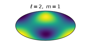
Choose a valid degree and order: 0 <= ell < L, and -ell <= m <= ell.

ell = 2
m = 1

# Use S2FFT's helper function to get the coefficient array shape described above.
flm_shape = s2fft.sampling.s2_samples.flm_shape(L)

# Set all coefficients to zero, then set f_{ell m} = 1.
flm = np.zeros(flm_shape, dtype=np.complex128)
flm[ell, m + L - 1] = 1.0

Since \(f_{\ell m}=1\) is the only non-zero coefficient, the spherical harmonic expansion reduces to

\[f(\theta,\phi) = 1 \cdot Y_{\ell m}(\theta,\phi) = Y_{\ell m}(\theta,\phi).\]

The inverse transform therefore evaluates the chosen basis function at the MW sample locations.

An individual spherical harmonic is generally complex-valued, so we set reality=False.

y_ell_m = s2fft.inverse(
    flm,
    L=L,
    sampling=sampling,
    method="jax",
    reality=False,
)

Spherical harmonics are generally complex-valued, so we visualise the real part.

fig, ax = plt.subplots(
    figsize=(3, 1.5),
    subplot_kw={"projection": ccrs.Mollweide()},
)

ax.imshow(
    y_ell_m.real,
    transform=ccrs.PlateCarree(),
    cmap="viridis",
)
ax.set_title(rf"$\ell={ell},\ m={m}$")

fig.tight_layout()
plt.show()

Visualising the basis

We can repeat the same construction, setting one coefficient to one and all remaining coefficients to zero, for every valid degree and order \((\ell,m)\) up to a chosen maximum degree.

max_degree = 3
ell_values = np.arange(max_degree + 1)
m_values = np.arange(-max_degree, max_degree + 1)

fig, axes = plt.subplots(
    len(ell_values),
    len(m_values),
    figsize=(16, 8),
    subplot_kw={"projection": ccrs.Mollweide()},
)

for ell in ell_values:
    for m in m_values:
        ax = axes[ell, m + max_degree]

        # Hide positions that do not correspond to a valid order.
        if abs(m) > ell:
            ax.set_axis_off()
            continue

        flm = np.zeros(flm_shape, dtype=np.complex128)
        flm[ell, m + L - 1] = 1.0

        y_ell_m = s2fft.inverse(
            flm,
            L=L,
            sampling=sampling,
            method="jax",
            reality=False,
        )

        ax.imshow(
            y_ell_m.real,
            transform=ccrs.PlateCarree(),
            cmap="viridis",
        )
        ax.set_title(rf"$\ell={ell},\ m={m}$", fontsize=9)

fig.tight_layout()
plt.show()

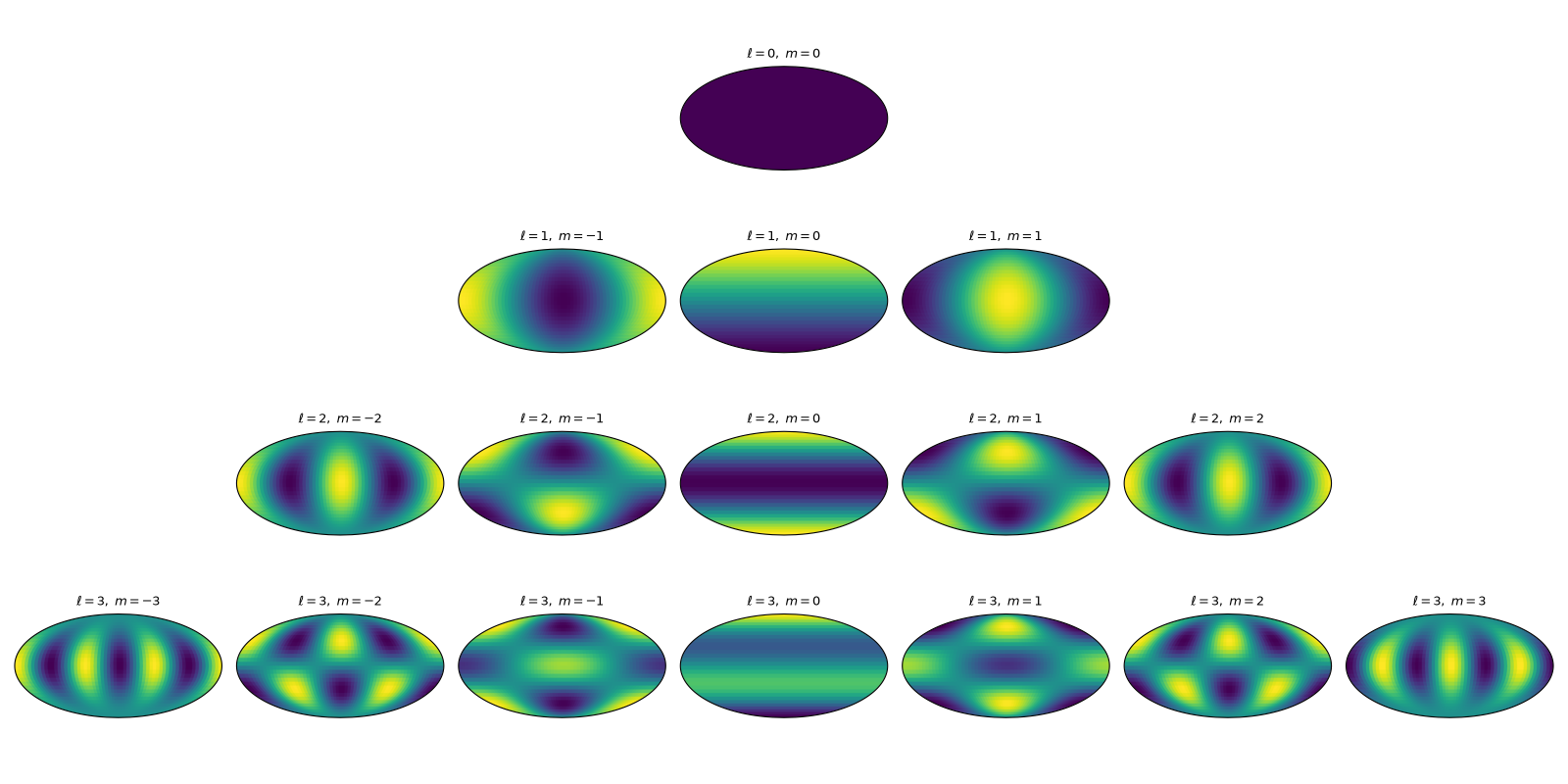
Moving down the rows increases \(\ell\), producing finer angular structure. Moving across a row changes \(m\). Increasing \(|m|\) produces more variation with longitude. When \(m=0\), the harmonic does not vary with longitude.

Decomposing a signal into spherical harmonics

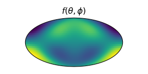
A band-limited signal is a weighted sum of spherical harmonic basis functions. To demonstrate this, we construct a signal with three non-zero coefficients:

\[f(\theta, \phi) = Y_{0,0}(\theta,\phi) + 0.8Y_{2,1}(\theta,\phi) - 0.4Y_{3,-2}(\theta,\phi).\]

The inverse transform evaluates this weighted sum at the MW sampling nodes.

signal_flm = np.zeros(flm_shape, dtype=np.complex128)
signal_flm[0, 0 + L - 1] = 1.0
signal_flm[2, 1 + L - 1] = 0.8
signal_flm[3, -2 + L - 1] = -0.4

signal = s2fft.inverse(
    signal_flm,
    L=L,
    sampling=sampling,
    method="jax",
    reality=False,
)

These coefficients do not satisfy conjugate symmetry, so the resulting signal is complex-valued. We visualise its real part below.

fig, ax = plt.subplots(
    figsize=(3, 1.5),
    subplot_kw={"projection": ccrs.Mollweide()},
)

ax.imshow(
    signal.real,
    transform=ccrs.PlateCarree(),
    cmap="viridis",
)
ax.set_title(r"$f(\theta,\phi)$")

fig.tight_layout()
plt.show()

Recovering the spherical harmonic coefficients

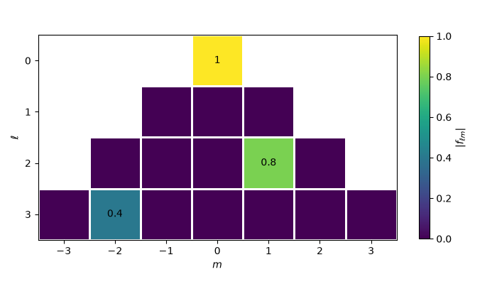
Starting from the sampled signal, the forward transform recovers its spherical harmonic coefficients, which are the weights of the basis functions.

recovered_flm = s2fft.forward(
    signal,
    L=L,
    sampling=sampling,
    method="jax",
    reality=False,
)

We display the magnitudes of the recovered coefficients up to degree three. The non-zero entries should occur at the same degree and order pairs used to construct the signal.

coefficient_magnitudes = np.abs(
    recovered_flm[: max_degree + 1, L - 1 - max_degree : L + max_degree]
)

# Leave invalid coefficients blank
coefficient_magnitudes[abs(m_values[None]) > ell_values[:, None]] = np.nan

fig, ax = plt.subplots(figsize=(7, 4))
im = ax.pcolormesh(
    m_values,
    ell_values,
    coefficient_magnitudes,
    cmap="viridis",
    edgecolors="white",
    linewidth=2,
)

# Label the non-zero coefficients
non_zero = ~np.isclose(np.nan_to_num(coefficient_magnitudes), 0)
for ell, m_index in np.argwhere(non_zero):
    ax.text(
        m_values[m_index],
        ell,
        f"{coefficient_magnitudes[ell, m_index]:.2g}",
        ha="center",
        va="center",
    )

ax.invert_yaxis()
ax.set(aspect=1, xlabel=r"$m$", ylabel=r"$\ell$", xticks=m_values, yticks=ell_values)
fig.colorbar(im, ax=ax, label=r"$|f_{\ell m}|$", shrink=0.8)

fig.tight_layout()
plt.show()

Finally, we compare the recovered coefficients with the original coefficients. For the MW sampling scheme, the error should be close to machine precision.

max_error = np.max(np.abs(recovered_flm - signal_flm))
print(f"Maximum coefficient error: {max_error:.2e}")

Maximum coefficient error: 7.08e-15