Solving Poisson’s equation on the sphere

Poisson’s equation relates a scalar field to a known source through the spherical Laplacian. In harmonic space, the spherical Laplacian becomes a simple multiplication, so the equation can be solved one coefficient at a time.

This tutorial uses S2FFT to solve Poisson’s equation on the unit sphere and compares the numerical solution with a known exact solution.

If you are working on this notebook in Google Colab, you will need to have Google Colab install cartopy and s2fft. You can do this by adding a cell to the top of the notebook with the following content:

!pip install cartopy s2fft &> /dev/null

and then running that cell.

Poisson’s equation on the sphere

Consider an unknown scalar field \(u(\theta,\phi)\) on the unit sphere, where \(\theta \in [0,\pi]\) is colatitude and \(\phi \in [0,2\pi)\) is longitude. Poisson’s equation is

\[\Delta_{\mathbb{S}^2} u = f,\]

where \(f(\theta,\phi)\) is a known source and \(\Delta_{\mathbb{S}^2}\) is the Laplace–Beltrami operator, the spherical counterpart of the usual Laplacian.

In spherical coordinates,

\[\Delta_{\mathbb{S}^{2}} u = \frac{1}{\sin\theta} \frac{\partial}{\partial\theta} \left(\sin\theta \frac{\partial u}{\partial\theta}\right) + \frac{1}{\sin^{2}\theta} \frac{\partial^{2}u}{\partial\phi^{2}}.\]

Poisson’s equation on the sphere arise in many settings, including geophysics, astrophysics, and fluid dynamics.

Harmonic space

Spherical harmonics are eigenfunctions of the Laplace–Beltrami operator:

\[\Delta_{\mathbb{S}^2} Y_{\ell m} = -\ell (\ell+1) Y_{\ell m}.\]

Expanding \(u\) and \(f\) in spherical harmonics therefore turns Poisson’s equation into a separate algebraic equation for each harmonic coefficient:

\[-\ell (\ell+1) u_{\ell m} = f_{\ell m}.\]

For every coefficient with \(\ell \geq 1\), the solution is

\[u_{\ell m} = -\frac{f_{\ell m}}{\ell(\ell+1)}.\]

The constant mode \(\ell = 0\) has eigenvalue zero because the Laplacian of a constant is zero. A solution therefore exists only if \(f_{00}=0\), meaning that the source has zero mean. Since adding any constant to \(u\) gives another solution, we select the zero-mean solution by setting \(u_{00} = 0\).

import jax

jax.config.update("jax_enable_x64", True)

import cartopy.crs as ccrs
import numpy as np
from matplotlib import pyplot as plt

import s2fft

L = 32
sampling = "mw"

Constructing a test problem

To test the numerical solution, we begin with a known exact solution,

\[u(\theta,\phi) = \sin\theta \cos\phi + \frac{1}{2} \left(3\cos^{2}\theta-1\right).\]

The first term contains only spherical harmonics of degree \(\ell = 1\), while the second contains only degree \(\ell = 2\). Since the spherical Laplacian acts on a mode of degree \(\ell\) as

\[\Delta_{\mathbb{S}^2} Y_{\ell m} = -\ell (\ell+1) Y_{\ell m},\]

it multiplies the first term by \(-2\) and the second by \(-6\).

The corresponding source is therefore

\[f(\theta,\phi) = -2 \sin\theta \cos\phi - 3 \left(3\cos^{2}\theta-1\right).\]

Both \(u\) and \(f\) have zero mean and contain only degrees up to \(\ell = 2\). They can therefore be represented exactly at any band-limit \(L \geq 3\), up to machine precision.

theta_values = s2fft.sampling.s2_samples.thetas(L, sampling)
phi_values = s2fft.sampling.s2_samples.phis_equiang(L, sampling)
theta_grid, phi_grid = np.meshgrid(theta_values, phi_values, indexing="ij")
longitude_grid = np.rad2deg(phi_grid)
latitude_grid = 90 - np.rad2deg(theta_grid)

exact_solution = np.sin(theta_grid) * np.cos(phi_grid) + 0.5 * (
    3 * np.cos(theta_grid) ** 2 - 1
)
source = -2 * np.sin(theta_grid) * np.cos(phi_grid) - 3 * (
    3 * np.cos(theta_grid) ** 2 - 1
)

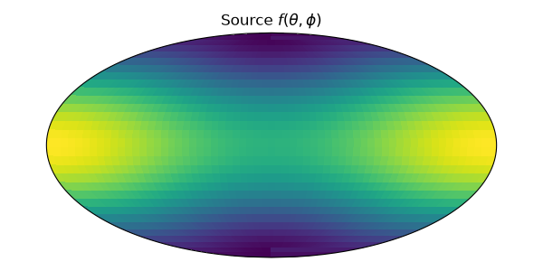
Visualising the source

The source \(f\) is the input to the Poisson problem.

fig, ax = plt.subplots(
    figsize=(6, 3),
    subplot_kw={"projection": ccrs.Mollweide()},
)

ax.pcolormesh(
    longitude_grid,
    latitude_grid,
    source,
    transform=ccrs.PlateCarree(),
    cmap="viridis",
)
ax.set_title(r"Source $f(\theta,\phi)$")

fig.tight_layout()
plt.show()

Transforming the source to harmonic space

The forward transform decomposes the sampled source into spherical harmonic coefficients \(f_{\ell m}\).

source_flm = np.asarray(
    s2fft.forward(
        source,
        L=L,
        sampling=sampling,
        method="jax",
        reality=True,
    )
)

Solving in harmonic space

We divide each coefficient with \(\ell\geq 1\) by the corresponding Laplacian eigenvalue. The coefficient array is initially zero, so its \(\ell=0\) row remains zero and selects the zero-mean solution.

ell_values = np.arange(L).reshape((L, 1))
laplacian_eigenvalues = -ell_values * (ell_values + 1)

solution_flm = np.zeros_like(source_flm)
solution_flm[1:] = source_flm[1:] / laplacian_eigenvalues[1:]

Visualising the coefficient operation

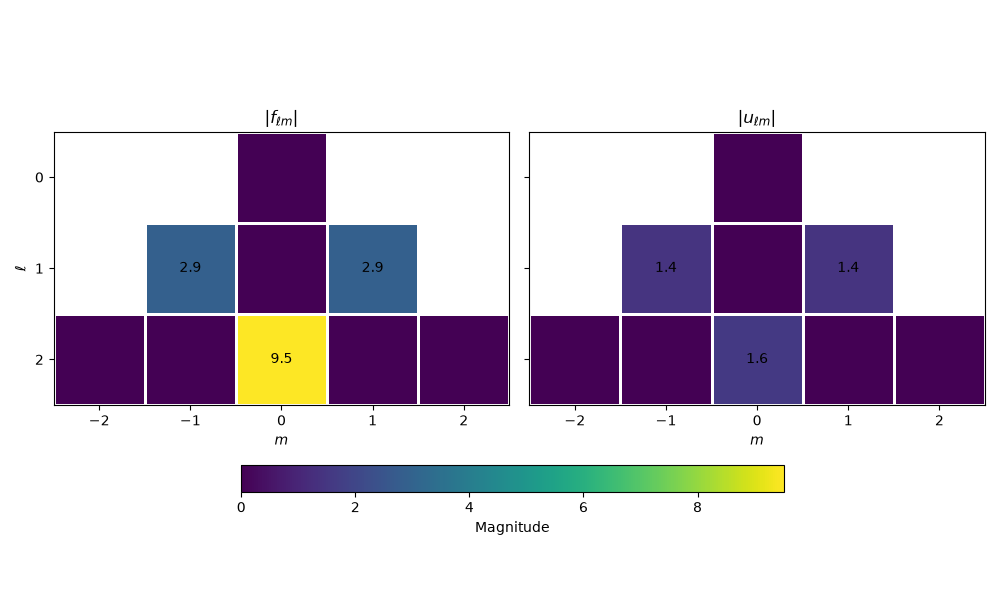
The heatmaps below compare the coefficients of the source and solution.

Solving Poisson’s equation leaves each coefficient at the same \((\ell,m)\) and divides it by the corresponding Laplacian eigenvalue \(-\ell(\ell+1)\). The solution therefore contains the same harmonic modes as the source, but with different magnitudes.

max_degree = 2
display_ell_values = np.arange(max_degree + 1)
display_m_values = np.arange(-max_degree, max_degree + 1)

coefficient_magnitudes = (
    np.abs(source_flm[: max_degree + 1, L - 1 - max_degree : L + max_degree]),
    np.abs(solution_flm[: max_degree + 1, L - 1 - max_degree : L + max_degree]),
)

# Leave entries that do not correspond to valid coefficients blank
invalid_coefficients = np.abs(
    display_m_values.reshape(1, 2 * max_degree + 1)
) > display_ell_values.reshape(max_degree + 1, 1)

for magnitudes in coefficient_magnitudes:
    magnitudes[invalid_coefficients] = np.nan

titles = (r"$|f_{\ell m}|$", r"$|u_{\ell m}|$")

fig, axes = plt.subplots(1, 2, figsize=(10, 6), sharex=True, sharey=True)

max_magnitude = max(np.nanmax(magnitudes) for magnitudes in coefficient_magnitudes)

for ax, magnitudes, title in zip(axes, coefficient_magnitudes, titles, strict=True):
    image = ax.pcolormesh(
        display_m_values,
        display_ell_values,
        magnitudes,
        cmap="viridis",
        vmin=0,
        vmax=max_magnitude,
        edgecolors="white",
        linewidth=2,
    )

    ax.set(
        title=title,
        xlabel=r"$m$",
        xticks=display_m_values,
        yticks=display_ell_values,
        aspect=1,
    )

    # Label non-zero coefficients
    non_zero = np.logical_not(np.isclose(np.nan_to_num(magnitudes), 0))
    for ell_index, m_index in np.argwhere(non_zero):
        ax.text(
            display_m_values[m_index],
            display_ell_values[ell_index],
            f"{magnitudes[ell_index, m_index]:.2g}",
            ha="center",
            va="center",
        )

axes[0].invert_yaxis()
axes[0].set_ylabel(r"$\ell$")

fig.colorbar(image, ax=axes, label="Magnitude", orientation="horizontal", shrink=0.7)

fig.tight_layout(rect=[0, 0.3, 1, 1])
plt.show()

Transforming back to the sphere

The inverse transform evaluates the solution at the original MW sample locations.

solution = np.asarray(
    s2fft.inverse(
        solution_flm,
        L=L,
        sampling=sampling,
        method="jax",
        reality=True,
    )
)

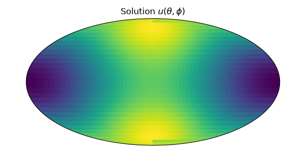
Visualising the solution

The spectral solution should agree with the exact solution.

fig, ax = plt.subplots(
    figsize=(6, 3),
    subplot_kw={"projection": ccrs.Mollweide()},
)

ax.pcolormesh(
    longitude_grid,
    latitude_grid,
    solution,
    transform=ccrs.PlateCarree(),
    cmap="viridis",
)
ax.set_title(r"Solution $u(\theta,\phi)$")

fig.tight_layout()
plt.show()

Checking the numerical accuracy

Finally, we compare the recovered solution with the exact solution. We also check how closely the recovered coefficients satisfy Poisson’s equation. In harmonic space, the residual is

\[r_{\ell m} = -\ell (\ell+1) u_{\ell m} - f_{\ell m}.\]

Since the test problem is band-limited and the MW sampling theorem applies, both the solution error and the residual should be close to machine precision.

absolute_error = np.abs(solution - exact_solution)

# Apply the spherical Laplacian to the recovered solution coefficients
laplacian_solution_flm = laplacian_eigenvalues * solution_flm

maximum_solution_error = np.max(absolute_error)
maximum_spectral_residual = np.max(np.abs(laplacian_solution_flm - source_flm))

print(f"Maximum solution error: {maximum_solution_error:.2e}")
print(f"Maximum spectral residual: {maximum_spectral_residual:.2e}")

Maximum solution error: 1.44e-15
Maximum spectral residual: 1.66e-15