Spatial derivatives of spherical signals

Spherical harmonic coefficients provide an accurate way to differentiate band-limited signals on the sphere. Instead of approximating a derivative from neighbouring samples, we differentiate the spherical harmonic expansion and then transform the result back to the sampling grid.

This tutorial computes derivatives with respect to colatitude and longitude and compares them with the exact derivatives of a known test signal.

If you are working on this notebook in Google Colab, you will need to have Google Colab install s2fft. You can do this by adding a cell to the top of the notebook with the following content:

!pip install cartopy s2fft &> /dev/null

and then running that cell.

Coordinate derivatives on the sphere

A scalar signal on the unit sphere is written as \(f(\theta,\phi)\), where \(\theta \in [0,\pi]\) is colatitude and \(\phi \in [0,2\pi)\) is longitude. Its surface gradient is

\[\nabla_{\mathbb{S}^2} f = \boldsymbol{e}_{\theta} \frac{\partial f}{\partial \theta} + \boldsymbol{e}_{\phi} \frac{1}{\sin \theta} \frac{\partial f}{\partial \phi},\]

where \(\boldsymbol{e}_{\theta}\) and \(\boldsymbol{e}_{\phi}\) are unit vectors in the colatitude and longitude directions, respectively. The factor \(1/\sin\theta\) accounts for the variation in physical distance associated with a change in longitude across the sphere.

We first compute the two coordinate derivatives \(\partial f/\partial\theta\) and \(\partial f / \partial\phi\). These derivatives are also fundamental building blocks for spectral methods used to solve partial differential equations on the sphere, with applications in atmospheric and ocean modelling.

import jax

jax.config.update("jax_enable_x64", True)

import cartopy.crs as ccrs
import numpy as np
from matplotlib import pyplot as plt

import s2fft

L = 32
sampling = "mw"

A band-limited signal

We use the real-valued signal

\[f(\theta,\phi) = \sin\theta\cos\phi + \frac{1}{2} \left(3\cos^{2}\theta-1 \right).\]

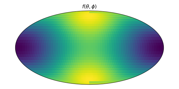
The first and second terms contain spherical harmonic modes of degrees one and two, respectively, so the signal has no harmonic content above degree two and is band-limited. Its exact coordinate derivatives are:

\[\frac{\partial f}{\partial \theta} = \cos\theta \cos\phi - 3 \sin\theta \cos\theta,\]

\[\frac{\partial f}{\partial \phi} = -\sin\theta \sin\phi.\]

theta_values = s2fft.sampling.s2_samples.thetas(L, sampling)
phi_values = s2fft.sampling.s2_samples.phis_equiang(L, sampling)
theta_grid, phi_grid = np.meshgrid(theta_values, phi_values, indexing="ij")
longitude_grid = np.rad2deg(phi_grid)
latitude_grid = 90 - np.rad2deg(theta_grid)

signal = np.sin(theta_grid) * np.cos(phi_grid) + 0.5 * (3 * np.cos(theta_grid) ** 2 - 1)

exact_colatitude_derivative = np.cos(theta_grid) * np.cos(phi_grid) - 3 * np.sin(
    theta_grid
) * np.cos(theta_grid)
exact_longitude_derivative = -np.sin(theta_grid) * np.sin(phi_grid)

Visualising the signal

We first visualise the sampled signal that will be differentiated.

fig, ax = plt.subplots(
    figsize=(6, 3),
    subplot_kw={"projection": ccrs.Mollweide()},
)

ax.pcolormesh(
    longitude_grid,
    latitude_grid,
    signal,
    transform=ccrs.PlateCarree(),
    cmap="viridis",
)

ax.set_title(r"$f(\theta,\phi)$")

fig.tight_layout()
plt.show()

Transforming to harmonic space

The forward transform decomposes the sampled signal into spherical harmonic coefficients \(f_{\ell m}\), which are used to compute the coordinate derivatives in harmonic space.

flm = np.asarray(
    s2fft.forward(
        signal,
        L=L,
        sampling=sampling,
        method="jax",
        reality=True,
    )
)

Differentiating with respect to longitude

The longitude dependence of a spherical harmonic is \(\exp(i m\phi)\). Therefore,

\[\frac{\partial}{\partial\phi}Y_{\ell m}(\theta,\phi) = im Y_{\ell m}(\theta,\phi).\]

Hence, the longitude derivative of the signal can be computed directly in harmonic space by multiplying each coefficient of order \(m\) by \(i m\).

m_values = np.arange(-L + 1, L)
longitude_derivative_flm = 1j * m_values * flm

longitude_derivative = np.asarray(
    s2fft.inverse(
        longitude_derivative_flm,
        L=L,
        sampling=sampling,
        method="jax",
        reality=True,
    )
)

Differentiating with respect to colatitude

Differentiation with respect to colatitude couples spherical harmonics with neighbouring degrees.

It is convenient to first consider the scaled derivative \(\sin\theta\ \frac{\partial Y_{\ell m}}{\partial\theta}\), which satisfies

\[\sin\theta \frac{\partial Y_{\ell m}}{\partial\theta} = \ell\epsilon_{\ell+1,m} Y_{\ell+1,m} - (\ell+1)\epsilon_{\ell m} Y_{\ell-1,m},\]

where the coupling factor is

\[\epsilon_{\ell m} = \sqrt{\frac{\ell^{2}-m^{2}}{4\ell^{2}-1}}.\]

Applying this relation to the harmonic expansion and collecting the coefficient of each \(Y_{\ell m}\) gives

\[\left(\sin\theta\frac{\partial f}{\partial\theta}\right)_{\ell m} = (\ell-1)\epsilon_{\ell m}f_{\ell-1,m} - (\ell+2)\epsilon_{\ell+1,m}f_{\ell+1,m}.\]

Thus, the coefficient at degree \(\ell\) receives contributions from the original coefficients at degrees \(\ell-1\) and \(\ell+1\). A more detailed derivation is given in the SpeedyWeather documentation on meridional derivatives. Note that the SpeedyWeather documentation is expressed using in terms of the latitude rather than the colatitude so the equations derived there do not exactly match the equations used here.

For a general signal with non-zero coefficients at the highest represented degree \(\ell=L-1\), the recurrence can generate a contribution at degree \(\ell=L\). In that case, the working band-limit must be increased before applying the recurrence.

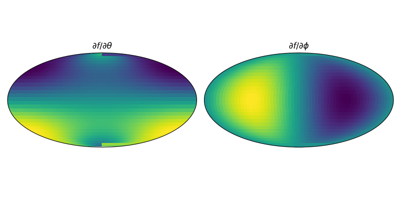
We reconstruct the scaled derivative and divide by \(\sin\theta\) to recover \(\frac{\partial f}{\partial\theta}\). The final MW ring lies at the south pole, where this coordinate derivative is undefined in general, so it is left blank.

ell_values = np.arange(L).reshape((L, 1))

# Invalid pairs with |m| > ell, and ell = 0, have epsilon = 0
epsilon = np.sqrt(
    np.maximum(ell_values**2 - m_values**2, 0) / np.maximum(4 * ell_values**2 - 1, 1)
)

# Align each output degree with the neighbouring input degree used in the recurrence
scaled_colatitude_derivative_flm = np.zeros_like(flm)
# Target degrees ell = 1, ..., L-1 receive contributions from degree ell-1
scaled_colatitude_derivative_flm[1:] += (ell_values[1:] - 1) * epsilon[1:] * flm[:-1]
# Target degrees ell = 0, ..., L-2 receive contributions from degree ell+1
scaled_colatitude_derivative_flm[:-1] -= (ell_values[:-1] + 2) * epsilon[1:] * flm[1:]

scaled_colatitude_derivative = np.asarray(
    s2fft.inverse(
        scaled_colatitude_derivative_flm,
        L=L,
        sampling=sampling,
        method="jax",
        reality=True,
    )
)

colatitude_derivative = scaled_colatitude_derivative.copy()
colatitude_derivative[:-1] /= np.sin(theta_values[:-1].reshape((-1, 1)))
colatitude_derivative[-1] = np.nan

Visualising the coefficient operations

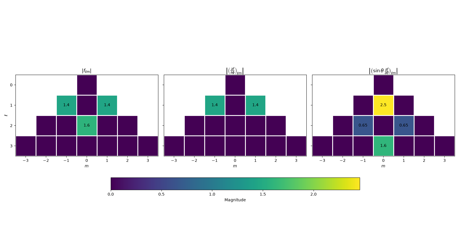
The heatmaps below compare the coefficients of the signal, the longitude derivative, and the scaled colatitude derivative.

Longitude differentiation leaves every coefficient at the same \((\ell,m)\) and multiplies it by \(i m\). In contrast, colatitude differentiation leaves \(m\) unchanged but moves information between neighbouring degrees \(\ell-1\) and \(\ell+1\).

max_degree = 3
display_ell_values = np.arange(max_degree + 1)
display_m_values = np.arange(-max_degree, max_degree + 1)

coefficient_magnitudes = [
    np.abs(flm[: max_degree + 1, L - 1 - max_degree : L + max_degree]),
    np.abs(
        longitude_derivative_flm[: max_degree + 1, L - 1 - max_degree : L + max_degree]
    ),
    np.abs(
        scaled_colatitude_derivative_flm[
            : max_degree + 1, L - 1 - max_degree : L + max_degree
        ]
    ),
]

# Leave entries that do not correspond to valid coefficients blank
invalid_coefficients = np.abs(
    display_m_values.reshape((1, -1))
) > display_ell_values.reshape((-1, 1))
for magnitudes in coefficient_magnitudes:
    magnitudes[invalid_coefficients] = np.nan

titles = (
    r"$|f_{\ell m}|$",
    r"$\left|\left(\frac{\partial f}{\partial\phi}\right)_{\ell m}\right|$",
    r"$\left|\left(\sin\theta\,\frac{\partial f}{\partial\theta}\right)_{\ell m}\right|$",
)

fig, axes = plt.subplots(1, 3, figsize=(16, 8), sharex=True, sharey=True)

max_magnitude = max(np.nanmax(magnitudes) for magnitudes in coefficient_magnitudes)

for ax, magnitudes, title in zip(axes, coefficient_magnitudes, titles, strict=False):
    image = ax.pcolormesh(
        display_m_values,
        display_ell_values,
        magnitudes,
        cmap="viridis",
        vmin=0,
        vmax=max_magnitude,
        edgecolors="white",
        linewidth=2,
    )
    ax.set(
        title=title,
        xlabel=r"$m$",
        xticks=display_m_values,
        yticks=display_ell_values,
        aspect=1,
    )

    # Label non-zero coefficients
    non_zero = np.logical_not(np.isclose(np.nan_to_num(magnitudes), 0))
    for ell_index, m_index in np.argwhere(non_zero):
        ax.text(
            display_m_values[m_index],
            display_ell_values[ell_index],
            f"{magnitudes[ell_index, m_index]:.2g}",
            ha="center",
            va="center",
        )

axes[0].invert_yaxis()
axes[0].set_ylabel(r"$\ell$")
fig.colorbar(image, ax=axes, label="Magnitude", orientation="horizontal", shrink=0.7)

fig.tight_layout(rect=[0, 0.3, 1, 1])
plt.show()

Visualising the derivatives

The two spectral derivatives are shown below. The undefined south-pole row of the colatitude derivative is left blank.

fields = colatitude_derivative, longitude_derivative
titles = r"$\partial f / \partial\theta$", r"$\partial f / \partial\phi$"

fig, axes = plt.subplots(
    1,
    2,
    figsize=(8, 4),
    subplot_kw={"projection": ccrs.Mollweide()},
)

for ax, field, title in zip(axes, fields, titles, strict=False):
    ax.pcolormesh(
        longitude_grid,
        latitude_grid,
        field,
        transform=ccrs.PlateCarree(),
        cmap="viridis",
    )
    ax.set_title(title)

fig.tight_layout()
plt.show()

Checking the accuracy

Finally, we compare the spectral derivatives with the exact derivatives of the test signal. Since the test signal is band-limited and the MW sampling theorem applies, both errors should be very small. The colatitude error excludes the south-pole ring and is slightly larger because division by \(\sin\theta\) amplifies numerical error near the poles.

colatitude_error = np.max(
    np.abs(colatitude_derivative[:-1] - exact_colatitude_derivative[:-1])
)
longitude_error = np.max(np.abs(longitude_derivative - exact_longitude_derivative))

print(f"Maximum colatitude derivative error: {colatitude_error:.2e}")
print(f"Maximum longitude derivative error: {longitude_error:.2e}")

Maximum colatitude derivative error: 6.07e-12
Maximum longitude derivative error: 1.75e-14